我们已经组装了完整的 Transformer 模型,现在我们准备好训练它进行神经机器翻译。为此,我们将使用一个训练数据集,其中包含简短的英语和德语句子对。我们还将重新审视掩蔽在训练过程中计算准确性和损失指标中的作用。
在本教程中,您将了解如何训练 Transformer 模型进行神经机器翻译。
完成本教程后,您将了解:
- 如何准备训练数据集。
- 如何将填充掩码应用于损失和准确性计算。
- 如何训练 Transformer 模型。
让我们开始吧。
教程概述
本教程分为四个部分;他们是:
- Transformer Architecture回顾
- 准备训练数据集
- 将填充掩码应用于损失和准确性计算
- 训练 Transformer 模型
先决条件
对于本教程,我们假设您已经熟悉:
- Transformer 模型背后的理论
- Transformer 模型的实现
Transformer Architecture回顾
回想一下,Transformer 架构遵循编码器-解码器结构:左侧的编码器负责将输入序列映射到连续表示序列;右侧的解码器接收编码器的输出以及前一时间步的解码器输出,以生成输出序列。
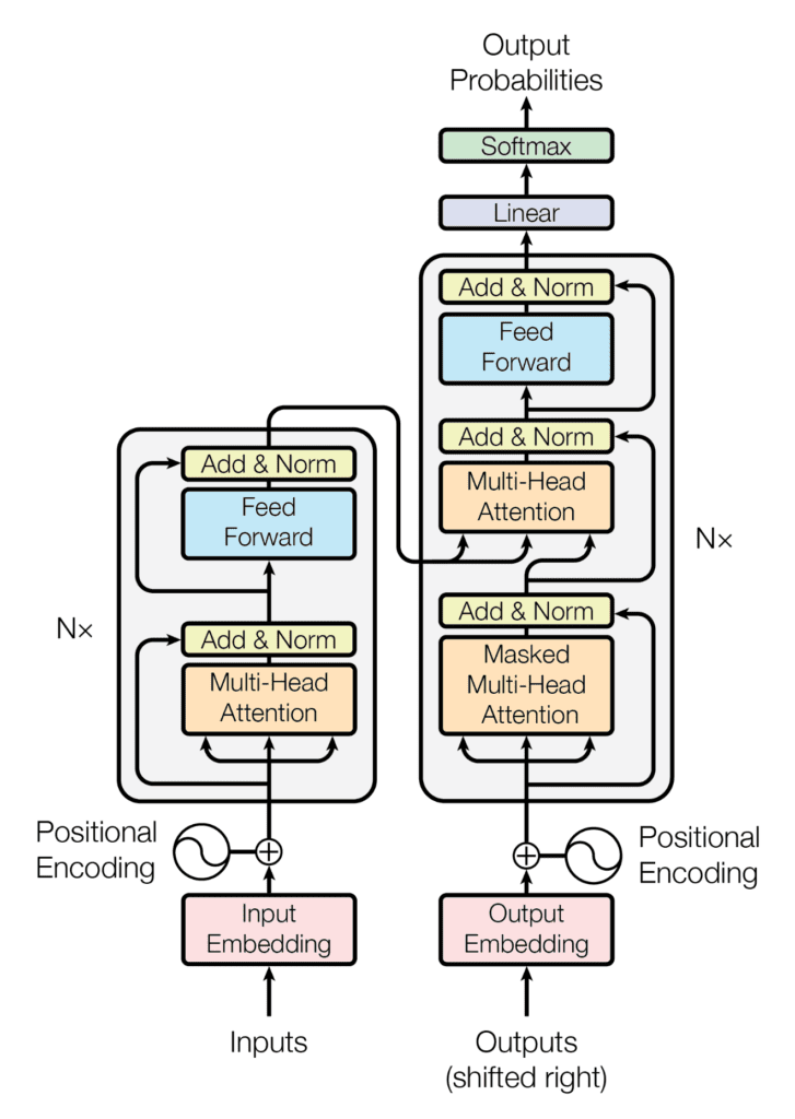
在生成输出序列时,Transformer 不依赖递归和卷积。
我们已经看到了如何实现完整的 Transformer 模型,现在我们将继续训练它以进行神经机器翻译。
让我们首先准备训练数据集。
准备训练数据集
为此,我们将参考之前的教程,该教程涵盖了与准备训练文本数据相关的材料。
我们还将使用包含简短英语和德语句子对的数据集,您可以在此处下载。这个特定的数据集已经通过删除不可打印和非字母字符以及标点符号进行了清理,并进一步将所有 Unicode 字符规范化为 ASCII,并将所有大写字母规范化为小写字母。因此,我们将跳过通常是数据准备过程一部分的清理步骤。但是,如果您使用的数据集不容易清理,您可以参考之前的教程以了解如何执行此操作。
让我们继续创建PrepareDataset实现以下步骤的类:
- 从指定的文件名加载数据集。
clean_dataset = load(open(filename, 'rb'))
- 从数据集中选择要使用的句子数。由于数据集很大,我们将减小其大小以限制训练时间。但是,您可以探索使用完整数据集作为本教程的扩展。
dataset = clean_dataset[:self.n_sentences, :]
- 将开始 (<START>) 和字符串结尾 (<EOS>) 标记附加到每个句子。例如,英语句子
i like to run, 现在变成了,<START> i like to run <EOS>。这也适用于其相应的德语翻译,ich gehe gerne joggen现在变成了,<START> ich gehe gerne joggen <EOS>。
for i in range(dataset[:, 0].size):
	dataset[i, 0] = "<START> " + dataset[i, 0] + " <EOS>"
dataset[i, 1] = "<START> " + dataset[i, 1] + " <EOS>"- 随机打乱数据集。
shuffle(dataset)
- 根据预定义的比率拆分混洗数据集。
train = dataset[:int(self.n_sentences * self.train_split)]
- 在将被输入编码器的文本序列上创建和训练一个分词器,并找到最长序列的长度以及词汇量大小。
enc_tokenizer = self.create_tokenizer(train[:, 0])
enc_seq_length = self.find_seq_length(train[:, 0])
enc_vocab_size = self.find_vocab_size(enc_tokenizer, train[:, 0])- 通过创建单词词汇表并将每个单词替换为其对应的词汇表索引,对将输入编码器的文本序列进行标记。<START> 和 <EOS> 标记也将构成该词汇表的一部分。每个序列也被填充到最大短语长度。
trainX = enc_tokenizer.texts_to_sequences(train[:, 0])
trainX = pad_sequences(trainX, maxlen=enc_seq_length, padding='post')
trainX = convert_to_tensor(trainX, dtype=int64)- 在将输入解码器的文本序列上创建和训练标记器,并找到最长序列的长度以及词汇量大小。
dec_tokenizer = self.create_tokenizer(train[:, 1])
dec_seq_length = self.find_seq_length(train[:, 1])
dec_vocab_size = self.find_vocab_size(dec_tokenizer, train[:, 1])- 对将输入解码器的文本序列重复类似的标记化和填充过程。
trainY = enc_tokenizer.texts_to_sequences(train[:, 1])
trainY = pad_sequences(trainY, maxlen=dec_seq_length, padding='post')
trainY = convert_to_tensor(trainY, dtype=int64)
完整的代码清单如下(有关详细信息,请参阅之前的教程):
from pickle import load
from numpy.random import shuffle
from keras.preprocessing.text import Tokenizer
from keras.preprocessing.sequence import pad_sequences
from tensorflow import convert_to_tensor, int64


class PrepareDataset:
	def __init__(self, **kwargs):
		super(PrepareDataset, self).__init__(**kwargs)
		self.n_sentences = 10000  # Number of sentences to include in the dataset
		self.train_split = 0.9  # Ratio of the training data split

	# Fit a tokenizer
	def create_tokenizer(self, dataset):
		tokenizer = Tokenizer()
		tokenizer.fit_on_texts(dataset)

		return tokenizer

	def find_seq_length(self, dataset):
		return max(len(seq.split()) for seq in dataset)

	def find_vocab_size(self, tokenizer, dataset):
		tokenizer.fit_on_texts(dataset)

		return len(tokenizer.word_index) + 1

	def __call__(self, filename, **kwargs):
		# Load a clean dataset
		clean_dataset = load(open(filename, 'rb'))

		# Reduce dataset size
		dataset = clean_dataset[:self.n_sentences, :]

		# Include start and end of string tokens
		for i in range(dataset[:, 0].size):
			dataset[i, 0] = "<START> " + dataset[i, 0] + " <EOS>"
			dataset[i, 1] = "<START> " + dataset[i, 1] + " <EOS>"

		# Random shuffle the dataset
		shuffle(dataset)

		# Split the dataset
		train = dataset[:int(self.n_sentences * self.train_split)]

		# Prepare tokenizer for the encoder input
		enc_tokenizer = self.create_tokenizer(train[:, 0])
		enc_seq_length = self.find_seq_length(train[:, 0])
		enc_vocab_size = self.find_vocab_size(enc_tokenizer, train[:, 0])

		# Encode and pad the input sequences
		trainX = enc_tokenizer.texts_to_sequences(train[:, 0])
		trainX = pad_sequences(trainX, maxlen=enc_seq_length, padding='post')
		trainX = convert_to_tensor(trainX, dtype=int64)

		# Prepare tokenizer for the decoder input
		dec_tokenizer = self.create_tokenizer(train[:, 1])
		dec_seq_length = self.find_seq_length(train[:, 1])
		dec_vocab_size = self.find_vocab_size(dec_tokenizer, train[:, 1])

		# Encode and pad the input sequences
		trainY = enc_tokenizer.texts_to_sequences(train[:, 1])
		trainY = pad_sequences(trainY, maxlen=dec_seq_length, padding='post')
		trainY = convert_to_tensor(trainY, dtype=int64)

		return trainX, trainY, train, enc_seq_length, dec_seq_length, enc_vocab_size, dec_vocab_size
在继续训练 Transformer 模型之前,我们先来看看PrepareDataset训练数据集中第一句话对应的类的输出:
# Prepare the training data
dataset = PrepareDataset()
trainX, trainY, train_orig, enc_seq_length, dec_seq_length, enc_vocab_size, dec_vocab_size = dataset('english-german-both.pkl')

print(train_orig[0, 0], '\n', trainX[0, :])
<START> did tom tell you <EOS>
tf.Tensor([ 1 25 4 97 5 2 0], shape=(7,), dtype=int64)(注意:由于数据集是随机打乱的,您可能会看到不同的输出。)
我们可以看到,最初,我们有一个三个词的句子(汤姆告诉过你),我们在其上附加了字符串的开始和结束标记,然后我们继续对其进行向量化(你可能会注意到 <START > 和 <EOS> 标记分别被分配词汇索引 1 和 2)。矢量化文本也用零填充,以便最终结果的长度与编码器的最大序列长度匹配:
print('Encoder sequence length:', enc_seq_length)
Encoder sequence length: 7
我们可以类似地检查输入解码器的相应目标数据:
print(train_orig[0, 1], '\n', trainY[0, :])
<START> hat tom es dir gesagt <EOS>
 tf.Tensor([  1  14   5   7  42 162   2   0   0   0   0   0], shape=(12,), dtype=int64)
这里,最终结果的长度与解码器的最大序列长度相匹配:
print('Decoder sequence length:', dec_seq_length)
Decoder sequence length: 12
将填充掩码应用于损失和准确性计算
回想一下,在编码器和解码器上使用填充掩码的重要性是确保我们刚刚附加到矢量化输入的零值不会与实际输入值一起处理。
这也适用于训练过程,其中需要填充掩码,以便在计算损失和准确性时不考虑目标数据中的零填充值。
我们先来看看损失的计算。
这将通过目标值和预测值之间的稀疏分类交叉熵损失函数来计算,然后乘以填充掩码,以便仅考虑有效的非零值。返回的损失是未屏蔽值的平均值:
def loss_fcn(target, prediction):
    # Create mask so that the zero padding values are not included in the computation of loss
    padding_mask = math.logical_not(equal(target, 0))
    padding_mask = cast(padding_mask, float32)

    # Compute a sparse categorical cross-entropy loss on the unmasked values
    loss = sparse_categorical_crossentropy(target, prediction, from_logits=True) * padding_mask

    # Compute the mean loss over the unmasked values
    return reduce_sum(loss) / reduce_sum(padding_mask)
为了计算准确度,首先比较预测值和目标值。预测的输出是一个大小的张量 ( batch_size , dec_seq_length , dec_vocab_size ),并且包含输出中标记的概率值(由解码器端的 softmax 函数生成)。为了能够与目标值进行比较,只考虑概率值最高的每个标记,并通过操作检索其字典索引:argmax(prediction, axis=2). 在应用填充掩码之后,返回的准确度是未掩码值的平均值:
def accuracy_fcn(target, prediction):
    # Create mask so that the zero padding values are not included in the computation of accuracy
    padding_mask = math.logical_not(math.equal(target, 0))

    # Find equal prediction and target values, and apply the padding mask
    accuracy = equal(target, argmax(prediction, axis=2))
    accuracy = math.logical_and(padding_mask, accuracy)

    # Cast the True/False values to 32-bit-precision floating-point numbers
    padding_mask = cast(padding_mask, float32)
    accuracy = cast(accuracy, float32)

    # Compute the mean accuracy over the unmasked values
    return reduce_sum(accuracy) / reduce_sum(padding_mask)
训练 Transformer 模型
让我们首先定义Vaswani 等人指定的模型和训练参数。(2017):
# Define the model parameters
h = 8  # Number of self-attention heads
d_k = 64  # Dimensionality of the linearly projected queries and keys
d_v = 64  # Dimensionality of the linearly projected values
d_model = 512  # Dimensionality of model layers' outputs
d_ff = 2048  # Dimensionality of the inner fully connected layer
n = 6  # Number of layers in the encoder stack

# Define the training parameters
epochs = 2
batch_size = 64
beta_1 = 0.9
beta_2 = 0.98
epsilon = 1e-9
dropout_rate = 0.1
(注意:我们在这里只考虑两个 epoch 以限制训练时间。但是,您可以探索进一步训练模型作为本教程的扩展。)
我们还需要实现一个学习率调度程序,它最初会线性增加第一个warmup_steps的学习率,然后按步数的平方根倒数按比例降低学习率。瓦萨尼等人。用以下公式表示:
学习率=d_model-0.5⋅分钟(步-0.5,步⋅warmup_steps-1.5)
class LRScheduler(LearningRateSchedule):
    def __init__(self, d_model, warmup_steps=4000, **kwargs):
        super(LRScheduler, self).__init__(**kwargs)

        self.d_model = cast(d_model, float32)
        self.warmup_steps = warmup_steps

    def __call__(self, step_num):

        # Linearly increasing the learning rate for the first warmup_steps, and decreasing it thereafter
        arg1 = step_num ** -0.5
        arg2 = step_num * (self.warmup_steps ** -1.5)

        return (self.d_model ** -0.5) * math.minimum(arg1, arg2)
该类的一个实例随后作为Adam 优化器LRScheduler的参数传递:learning_rate
optimizer = Adam(LRScheduler(d_model), beta_1, beta_2, epsilon)
接下来,我们将数据集拆分为批次,为训练做准备:
train_dataset = data.Dataset.from_tensor_slices((trainX, trainY))
train_dataset = train_dataset.batch(batch_size)
接下来是模型实例的创建:
training_model = TransformerModel(enc_vocab_size, dec_vocab_size, enc_seq_length, dec_seq_length, h, d_k, d_v, d_model, d_ff, n, dropout_rate)
在训练 Transformer 模型时,我们将编写自己的训练循环,其中包含我们之前实现的损失函数和准确率函数。
Tensorflow 2.0 中的默认运行时是eager execution,这意味着操作一个接一个地立即执行。Eager execution 简单直观,使调试更容易。然而,它的缺点是它无法利用使用图形执行运行代码所带来的全局性能优化。在图执行中,首先在执行张量计算之前构建图,这会产生计算开销。出于这个原因,大多数情况下建议将图执行用于大型模型训练,而不是用于小型模型训练,因为 Eager Execution 可能更适合执行更简单的操作。由于 Transformer 模型足够大,我们将应用图形执行来训练它。
为此,我们将按@function如下方式使用装饰器:
@function
def train_step(encoder_input, decoder_input, decoder_output):
    with GradientTape() as tape:

        # Run the forward pass of the model to generate a prediction
        prediction = training_model(encoder_input, decoder_input, training=True)

        # Compute the training loss
        loss = loss_fcn(decoder_output, prediction)

        # Compute the training accuracy
        accuracy = accuracy_fcn(decoder_output, prediction)

    # Retrieve gradients of the trainable variables with respect to the training loss
    gradients = tape.gradient(loss, training_model.trainable_weights)

    # Update the values of the trainable variables by gradient descent
    optimizer.apply_gradients(zip(gradients, training_model.trainable_weights))

    train_loss(loss)
train_accuracy(accuracy)通过添加@function装饰器,将张量作为输入的函数将编译为图形。如果@function装饰器被注释掉,则该函数会以急切执行的方式运行。
下一步是实现将调用上述train_step函数的训练循环。训练循环将迭代指定数量的 epoch 和数据集批次。对于每个批次,该train_step函数计算训练损失和准确度度量,并应用优化器更新可训练模型参数。还包括一个检查点管理器,以在每五个 epoch 后保存一个检查点:
train_loss = Mean(name='train_loss')
train_accuracy = Mean(name='train_accuracy')

# Create a checkpoint object and manager to manage multiple checkpoints
ckpt = train.Checkpoint(model=training_model, optimizer=optimizer)
ckpt_manager = train.CheckpointManager(ckpt, "./checkpoints", max_to_keep=3)

for epoch in range(epochs):

    train_loss.reset_states()
    train_accuracy.reset_states()

    print("\nStart of epoch %d" % (epoch + 1))

    # Iterate over the dataset batches
    for step, (train_batchX, train_batchY) in enumerate(train_dataset):

        # Define the encoder and decoder inputs, and the decoder output
        encoder_input = train_batchX[:, 1:]
        decoder_input = train_batchY[:, :-1]
        decoder_output = train_batchY[:, 1:]

        train_step(encoder_input, decoder_input, decoder_output)

        if step % 50 == 0:
            print(f'Epoch {epoch + 1} Step {step} Loss {train_loss.result():.4f} Accuracy {train_accuracy.result():.4f}')

    # Print epoch number and loss value at the end of every epoch
    print("Epoch %d: Training Loss %.4f, Training Accuracy %.4f" % (epoch + 1, train_loss.result(), train_accuracy.result()))

    # Save a checkpoint after every five epochs
    if (epoch + 1) % 5 == 0:
        save_path = ckpt_manager.save()
        print("Saved checkpoint at epoch %d" % (epoch + 1))
要记住的重要一点是,解码器的输入相对于编码器输入向右偏移一个位置。这个偏移背后的想法,结合解码器的第一个多头注意力块中的前瞻掩码,是为了确保对当前令牌的预测只能依赖于之前的令牌。
这种掩蔽与输出嵌入偏移一个位置的事实相结合,确保对位置 i 的预测只能依赖于位置小于 i 的已知输出。
–注意就是你所需要的,2017。
正是出于这个原因,编码器和解码器的输入以下列方式输入到 Transformer 模型中:
encoder_input = train_batchX[:, 1:]
decoder_input = train_batchY[:, :-1]
将完整的代码清单放在一起产生以下内容:
from tensorflow.keras.optimizers import Adam
from tensorflow.keras.optimizers.schedules import LearningRateSchedule
from tensorflow.keras.metrics import Mean
from tensorflow import data, train, math, reduce_sum, cast, equal, argmax, float32, GradientTape, TensorSpec, function, int64
from keras.losses import sparse_categorical_crossentropy
from model import TransformerModel
from prepare_dataset import PrepareDataset
from time import time


# Define the model parameters
h = 8  # Number of self-attention heads
d_k = 64  # Dimensionality of the linearly projected queries and keys
d_v = 64  # Dimensionality of the linearly projected values
d_model = 512  # Dimensionality of model layers' outputs
d_ff = 2048  # Dimensionality of the inner fully connected layer
n = 6  # Number of layers in the encoder stack

# Define the training parameters
epochs = 2
batch_size = 64
beta_1 = 0.9
beta_2 = 0.98
epsilon = 1e-9
dropout_rate = 0.1


# Implementing a learning rate scheduler
class LRScheduler(LearningRateSchedule):
    def __init__(self, d_model, warmup_steps=4000, **kwargs):
        super(LRScheduler, self).__init__(**kwargs)

        self.d_model = cast(d_model, float32)
        self.warmup_steps = warmup_steps

    def __call__(self, step_num):

        # Linearly increasing the learning rate for the first warmup_steps, and decreasing it thereafter
        arg1 = step_num ** -0.5
        arg2 = step_num * (self.warmup_steps ** -1.5)

        return (self.d_model ** -0.5) * math.minimum(arg1, arg2)


# Instantiate an Adam optimizer
optimizer = Adam(LRScheduler(d_model), beta_1, beta_2, epsilon)

# Prepare the training and test splits of the dataset
dataset = PrepareDataset()
trainX, trainY, train_orig, enc_seq_length, dec_seq_length, enc_vocab_size, dec_vocab_size = dataset('english-german-both.pkl')

# Prepare the dataset batches
train_dataset = data.Dataset.from_tensor_slices((trainX, trainY))
train_dataset = train_dataset.batch(batch_size)

# Create model
training_model = TransformerModel(enc_vocab_size, dec_vocab_size, enc_seq_length, dec_seq_length, h, d_k, d_v, d_model, d_ff, n, dropout_rate)


# Defining the loss function
def loss_fcn(target, prediction):
    # Create mask so that the zero padding values are not included in the computation of loss
    padding_mask = math.logical_not(equal(target, 0))
    padding_mask = cast(padding_mask, float32)

    # Compute a sparse categorical cross-entropy loss on the unmasked values
    loss = sparse_categorical_crossentropy(target, prediction, from_logits=True) * padding_mask

    # Compute the mean loss over the unmasked values
    return reduce_sum(loss) / reduce_sum(padding_mask)


# Defining the accuracy function
def accuracy_fcn(target, prediction):
    # Create mask so that the zero padding values are not included in the computation of accuracy
    padding_mask = math.logical_not(equal(target, 0))

    # Find equal prediction and target values, and apply the padding mask
    accuracy = equal(target, argmax(prediction, axis=2))
    accuracy = math.logical_and(padding_mask, accuracy)

    # Cast the True/False values to 32-bit-precision floating-point numbers
    padding_mask = cast(padding_mask, float32)
    accuracy = cast(accuracy, float32)

    # Compute the mean accuracy over the unmasked values
    return reduce_sum(accuracy) / reduce_sum(padding_mask)


# Include metrics monitoring
train_loss = Mean(name='train_loss')
train_accuracy = Mean(name='train_accuracy')

# Create a checkpoint object and manager to manage multiple checkpoints
ckpt = train.Checkpoint(model=training_model, optimizer=optimizer)
ckpt_manager = train.CheckpointManager(ckpt, "./checkpoints", max_to_keep=3)

# Speeding up the training process
@function
def train_step(encoder_input, decoder_input, decoder_output):
    with GradientTape() as tape:

        # Run the forward pass of the model to generate a prediction
        prediction = training_model(encoder_input, decoder_input, training=True)

        # Compute the training loss
        loss = loss_fcn(decoder_output, prediction)

        # Compute the training accuracy
        accuracy = accuracy_fcn(decoder_output, prediction)

    # Retrieve gradients of the trainable variables with respect to the training loss
    gradients = tape.gradient(loss, training_model.trainable_weights)

    # Update the values of the trainable variables by gradient descent
    optimizer.apply_gradients(zip(gradients, training_model.trainable_weights))

    train_loss(loss)
    train_accuracy(accuracy)


for epoch in range(epochs):

    train_loss.reset_states()
    train_accuracy.reset_states()

    print("\nStart of epoch %d" % (epoch + 1))

    start_time = time()

    # Iterate over the dataset batches
    for step, (train_batchX, train_batchY) in enumerate(train_dataset):

        # Define the encoder and decoder inputs, and the decoder output
        encoder_input = train_batchX[:, 1:]
        decoder_input = train_batchY[:, :-1]
        decoder_output = train_batchY[:, 1:]

        train_step(encoder_input, decoder_input, decoder_output)

        if step % 50 == 0:
            print(f'Epoch {epoch + 1} Step {step} Loss {train_loss.result():.4f} Accuracy {train_accuracy.result():.4f}')
            # print("Samples so far: %s" % ((step + 1) * batch_size))

    # Print epoch number and loss value at the end of every epoch
    print("Epoch %d: Training Loss %.4f, Training Accuracy %.4f" % (epoch + 1, train_loss.result(), train_accuracy.result()))

    # Save a checkpoint after every five epochs
    if (epoch + 1) % 5 == 0:
        save_path = ckpt_manager.save()
        print("Saved checkpoint at epoch %d" % (epoch + 1))

print("Total time taken: %.2fs" % (time() - start_time))
运行代码会产生与以下类似的输出(您可能会看到不同的损失和准确度值,因为我们是从头开始训练的,而训练时间取决于您可用于训练的计算资源):
Start of epoch 1
Epoch 1 Step 0 Loss 8.4525 Accuracy 0.0000
Epoch 1 Step 50 Loss 7.6768 Accuracy 0.1234
Epoch 1 Step 100 Loss 7.0360 Accuracy 0.1713
Epoch 1: Training Loss 6.7109, Training Accuracy 0.1924

Start of epoch 2
Epoch 2 Step 0 Loss 5.7323 Accuracy 0.2628
Epoch 2 Step 50 Loss 5.4360 Accuracy 0.2756
Epoch 2 Step 100 Loss 5.2638 Accuracy 0.2839
Epoch 2: Training Loss 5.1468, Training Accuracy 0.2908
Total time taken: 87.98s
代码在仅使用 CPU 的同一平台上单独使用 Eager Execution 运行需要 155.13 秒,这显示了使用图形执行的好处。
